|
ROBERT F. MULLIGAN
|
|

A Brief Introduction to
Econometrics
1.
The basic univariate model: Yt = a + bXt + et.
Y is called the left-hand-side variable, LHS variable, the dependent variable, or
the explained variable. X is the right-hand-side, RHS variable, dependent, or
explanatory variable. e is the residual, error, or disturbance term. The
expression (a + bXt) is called the fitted value of Y and is also
referred to as Y-hat. The regression calculates values of a and b, the
"regression coefficients," that best fit the data for X and Y (hence
regression is sometimes called "curve fitting,") by minimizing the
sum of squared residuals, ∑tet2 (or e'e
in vector notation.) This most basic and
commonly used regression technique is called ordinary least squares, OLS, OLSQ,
or LS.
To run a
regression in MS Excel 97, enter your data in a worksheet. Normally each
variable is placed in its own column, with the name of the variable and any
other information you may wish to place there, like units and data
transformations you performed (which are not used for computing the regression
coefficients), at the top of the column. Click on "Tools" in
the toolbar at the top of the screen to get the "Tools" menu, then go
down to the bottom and click on "Data Analysis." Scroll down
the "Data Analysis" window until you find "Regression,"
highlight it, and press "enter." You will be provided a dialog
box which enables you to set the range for each variable in the regression.
Y is the left-hand-side variable. Click on the Icon on the right side of
the window for the Y variable range (it looks like a little table with tiny
text windows - real cute.) Then highlight all the numerical values of the
LHS variable. The screen will show a dotted line around the numbers you
highlight. Press enter, and the dialog box will reappear with the range
of the LHS variable you selected. Repeat for the RHS variable. You
can highlight more than one column on the RHS to estimate a multivariate
regression. Make sure each variable has the same number of
observations. When you are satisfied with the Y and X ranges in the
dialog box, click on the "OK" button, and your output will appear on
a new sheet in your current worksheet.
2. The
basic univariate model in vector notation: y = Xβ + e where y is an (n x 1)
column vector of the different observations of the left-hand-side variable, X
is an (n x 2) matrix for which the first column is a column of ones
(representing the constant or intercept term) and the second column is a column
of the n observations of the right-hand-side variable, β is a (2 x 1) vector of estimated
coefficients (the intercept or constant, and the slope or X coefficient,) and e
is an (n x 1) vector of residuals or disturbance terms. This model is the same
as in part 1, and looks like this:
|
|
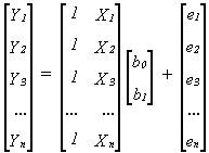
Note
that I have renamed the intercept b0 (instead of a) and the slope b1
(instead of just b).
In
MS Excel 97, you can force the regression line through the origin, setting a =
b0 = 0, by checking the "Constant is Zero" option
on the regression dialog box.
3.
The basic multivariate model (in vector notation): y = Xβ + e is the same as the simple univariate
case except that now X is an (n x k+1) matrix (called the observation or
data or independent variable matrix) consisting of a column of n ones
(representing the intercept) and k columns of n observations of the k
right-hand-side variables, and β is a (k+1 x 1)
column vector of estimated coefficients. This model has more than just one
explanatory or independent variable and looks like this:
|
|
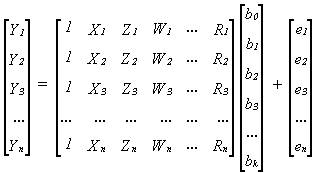
This
model can also be written as: Yt = b0 + b1Xt
+ b2Zt + b3Wt + b4Rt
+ et, supposing there are only four right-hand-side variables.
In
MS Excel 97, you estimate a multivariate regression by selecting an X range
with more than one column, which the software reads as more than one
variable. It is important each column has the same height, lined up row
by row, and that each column be adjacent.
4.
Non-linear regression: What if Y is a function of X, but not a linear
function of X? Then form second-order terms by squaring each X, and estimate
the regression as: Yt = a + bXt + cXt2
+ et. You can also cube X or raise it to any power you want. If it
is a multivariate regression, (with, say, X and Z as right-hand-side
variables,) you can also add cross-product terms (in this case XZ as well as X2
and Z2.)
You
could do this by creating new columns from your original X variables. Or
you could transform your data into logarithms.
5.
Some regression output:
MS Excel
97 provides three output tables whenever you run a regression.
Excel
Table 1: Regression Statistics
The first table gives statistics which measure the fit of the regression as a
whole. The multiple R is the coefficient of correlation between Y and
Y-hat. (For a univariate regression, with only one RHS variable, R is the
coefficient of correlation between X and Y). R is the square root of the R-squared, the
coefficient of determination. The range of R is between -1 and +1, so
R-squared ranges from 0 to 1. Theoretically, the adjusted R-squared, the
coefficient of determination adjusted for degrees of freedom, or R-bar-squared,
has the same range, but it can be negative when the number of coefficients
being estimated—that is, the number of RHS variables—is high compared to the
number of observations or sample size. R-squared = R-bar-squared = 1
indicate a perfect fit. The closer these are to one, the better the
regression fits the data. The standard error of the regression, which
should be as low as possible, and the number of observation are also provided.
Excel
Table 2: The F-Statistic
The second table, labeled ANOVA for "Analysis of Variance," computes
an F statistic which tests whether the estimated coefficients (the b's) are
jointly significantly different from zero. The last column in this table
gives the significance level of the F test, which should be less than or equal
to 5% (= 0.05) or some other arbitrarily chosen low percentage. The
table gives degrees of freedom ("df") and sums of squares
("SS") for the regression (SSR), the residuals or error terms (SSE),
and the total, for the LHS variable (SST). To get the SST, square each
observation of the LHS variable and add the squares. To get the SSE,
square each error term and add the squares. To get the SSR, subtract SSE
from SST, or square each value of Y-hat (the fitted values of Y) and add the
squares.
Next,
the table gives mean squares, which are the SSR and SSE divided by their
degrees of freedom. For the SSR, the df is the number of RHS variables
with coefficients being estimated, not including the constant. The
df for the SSE is the number of observations, minus the number of coefficients
being estimated, including the constant. The SSR and SSE df add up
to one less than the number of observations (1 - n), which is the SST df.
One degree of freedom is eaten up by the constant, which is why the SST df is
one less than the number of observations of each variable, as long as a
constant is included in the regression.
The
ratio of the two mean squares MSR/MSE is F-distributed under ideal
conditions. This is listed under F. MST is not used to calculate
the F statistic, so it is not listed in the ANOVA table. The F ratio
tests the joint hypothesis H0: (b1 = b2 = b3
= . . . = bk = 0), the null hypothesis that all the b
coefficients (except b0 the intercept or constant) are
jointly equal to zero. The significance level of the F ratio is greater than 5%
(or some other low value you choose) to accept (or "fail to
reject") the null hypothesis, which tells you the regression has no
explanatory power. The significance level of the F ratio is less than 5% (or
some other value you choose) to reject the null hypothesis, which tells you the
regression has some explanatory power.
Excel
Table 3: Estimated Coefficients and their t-Statistics
The third table provides (finally!) the estimated coefficients for the intercept
and each RHS X variable. Each coefficient has a standard error. The
t-statistic or t-ratio is the ratio of each coefficient divided by its standard
error. Each t-ratio is t-distributed under ideal conditions. Each t
test tests the null hypothesis H0: (bj = 0), that
each coefficient is equal to zero. The t-statistic independently tests
the significance of each estimated coefficient while the F jointly tests
whether they all work together. Usually
if any t-stats are greater than 2.00, the F statistic will also be
significant. The significance level of
the t ratio is greater than 5% (or some other low value you choose) to
accept (or "fail to reject") the null hypothesis, which tells you the
variable may be removed from the regression, so take it out and estimate the
regression without it. The significance level of the t ratio is less than 5%
(or some other value you choose) to reject the null hypothesis, which tells you
the variable may be kept.
In
addition to estimated coefficients for each variable and the intercept or
constant term, most regression softwares provide some or all of the following:
1.
Standard error (of a coefficient) tells you how likely the true or population
value of the estimated coefficient will lie within a certain distance from the
estimate (or sample value,) based on the dispersion of the data. The smaller
the better. The true value is about 67% likely to lie within plus or minus one
standard error from the estimated value, and about 95% likely to lie within
plus or minus two standard errors. MS Excel 97 provides this in the
coefficient estimate table.
2.
t-statistic (t-ratio): The estimated coefficient divided by its standard error.
The higher the better. If t exceeds 1, it is at least about 67% likely that the
true value of the coefficient is not zero, and if t exceeds 2, it is at least
about 95% likely. This tests the hypothesis that the true value of an estimated
coefficient is equal to zero, and that that variable should be deleted.
MS Excel 97 provides this next to the standard error in the coefficient
estimate table.
3.
Probability value of the t statistic (2-tailed significance level): Gives the
probability value of the computed t statistic from an internal table of the t
distribution. The lower the better. Less than .05 (or .10 or .01, this is
called an alpha or level of significance, which you choose) for statistically
significant coefficients.
4. R2
(Coefficient of determination): Ranges from 0 to 1. The higher the better.
Measures the % of variation in Y that is explained by variation in the
right-hand-side variables. In a univariate regression it is the square of the
coefficient of correlation (rXY) between X and Y. It is calculated
by this formula:
|
|
Y-bar is
the sample mean of Y, SSE means "sum of squared errors" (or sum of
squared residuals, e'e in vector
notation), and SST means "sum of squares total." SSR is the "sum
of squares regression," and they all fit into this identity: SST = SSR +
SSE. SSE can't be referred to as SSR (though, unfortunately, sometimes it is.)
To make things more confusing, SSR is also called the "explained sum of
squares" because it's what's explained by the regression, and SSE is also
known as the "unexplained sum of squares," because it's what's left
over. If the regression were a perfect fit, all the e's would be zero, and so
SSE would equal zero and R2 would equal one. (This would mean that
SSR = SST.) MS Excel 97 provides the R2 in the regression
statistics table, just under its square root, "Multiple R."
5.
Adjusted R2 (R2 adjusted for degrees of freedom, aka
R-bar-squared): Interpreted the same way as R2, but can be negative.
Should never be greater than R2. It is calculated by this formula:
|
|
The
formula is basically the same as for R2, but includes adjustments
for the size of the sample (n) and the number of coefficients being estimated
(k+1). MS Excel 97 provides this in the regression statistics table under
the R2.
6.
Durbin-Watson statistic (DW or d): Tests for serial correlation of residuals:
Serial correlation means that the error terms are systematically related
through time, and not statistically independent of each other. Theoretically
the errors should be white noise, or perfectly random. When they aren't, the
whole estimate's validity is questionable. DW is close to 2 in the absence of
serial correlation. Critical values for DW can be found in the (old)
Durbin-Watson or (newer) Savin-White tables in the back of most econometrics
texts. In cross-sectional data, serial correlation is called autocorrelation,
and can be solved by just scrambling the order of the data (basically you can
do this because the order of the observations wasn't important to start with.)
With time-series data—commonly used in macroeconomics—you can't change the
order, so you have two choices: difference your regression equation (see
below), or apply a correction for serial correlation of the error terms,
typically the Cochrane-Orcutt iterative correction (provided by MicroTSP) or
Beach-MacKinnon iterative maximum likelihood method (provided by TSP). MS
Excel 97 does not provide a test for serial correlation or an estimation
technique robust to serial correlation.
7.
Durbin's h and/or Durbin's h alternative: TSP provides this, but MicroTSP
doesn't (yet). It's an improved test statistic for serial correlation and should
be used in preference to DW whenever there are a large number of explanatory
variables, or when some of the explanatory variables are lagged values of Y.
TSP 4.2 prints out the probability, which you want to be less than the
significance level you choose, a = .10, .05, or .01. MS Excel 97 does not
provide a test for serial correlation. Too bad.
8. Log
likelihood (logarithm of the likelihood function): If n is the number of
observations of each variable in the regression, this is calculated by the formula:
|
|
The
larger L the better (consequently the larger logL the better) but this is only
meaningful when comparing two regressions: the one with the larger logL is the
better of the two. The difference of the logL's is chi-square distributed, and if
its probability value is below some critical significance level (a), usually
.05, the model with the lower likelihood is rejected. This is called a
likelihood ratio test because the test statistic (the difference between
logL's) is the log of a ratio. The formula used for the log likelihood is based
on the normal distribution; theoretically the distribution of the residuals
should become more nearly normal as the number of observations n approaches
infinity. Maximum likelihood estimation is an alternative technique to least
squares that chooses the estimated coefficients to make the residuals most
nearly normally distributed. Instead of minimizing the sum of squared
residuals, it maximizes the value of the normal likelihood function. The higher
logL is for a least squares estimate, the closer it is to the maximum
likelihood or ML estimate. It is not always useful to assume that residuals are
normally distributed, see sect. 7.5 below. MS Excel 97 does not provide
this.
9.
Standard error of the regression: Measures the magnitude of the residuals.
About 67% will lie between one standard error above zero and one below, and
about 95% will lie between plus or minus two standard errors. The smaller the
better. MS Excel 97 provides this in the first regression output table,
under "Standard Error."
10. Sum
of squared residuals: (e'e) This is what is minimized by a least squares
estimate. The smaller the better. MS Excel 97 provides this in the SS
column of the ANOVA table, under "Residual."
11. F
statistic (zero slopes): Tests whether the estimated values of the coefficients
are all significantly different from zero. Doesn't include the constant or
intercept. For a univariate regression is equal to the square of the t
statistic for the right-hand-side variable. The higher the better. You want the
probability value of the F statistic to be less than a = .10, .05, or .01. MS
Excel 97 provides the F statistic and its probability level at the far right of
the ANOVA table.
12.
Akaike Information Criterion (AIC): AIC
= ln(SSE/n) + 2k/n, where n is the number of observations or sample size, k is
the number of coefficients being estimated, including the constant if any, and
SSE is the sum of squared residuals from the regression, aka e'e.
The lower this number is, the more efficient the regression model is in
making use of the available information contained in the data to estimate the
regression coefficients. Note that the
formulas for the three information criteria are similar to the R-square.
R-square always increases when additional RHS variables are added. The information criteria attempt to measure
whether the information contained in additional RHS variables, which always
increases the R-square, is sufficient to warrant adding more variables to the
model. If adding a variable to the
regression results in the AIC falling, then add the variable. If removing a variable results in the AIC
falling, then remove the variable. The
AIC is automatically computed by Eviews, but not by MS Excel.
13. Schwarz Bayesian Information Criterion (SBIC
or SC): SBIC = ln(SSE/n) + (k
ln(n))/n. The SBIC is an alternative
approach to measuring the information efficiency of a regression model. SBIC is interpreted the same as the other
information criteria, but does not always give the same results. It is automatically computed by Eviews as
part of the regression output, but not by MS Excel.
14. Amemiya's Prediction Criterion (PC): Amemiya's PC = SSE(1 + k/n)/(n – k). Amemiya's PC is yet another approach to
measuring the information efficiency of a regression model. This is interpreted the same way as the AIC
or the SBIC, lower is better, but does not always give the same results. It is not computed by either Eviews or MS
Excel.
5.
The kinds of data.
a.
Time-series data: A different value of each variable is observed for each
period of time, e.g., annually, quarterly, monthly, weekly, daily, etc. Gross
domestic product (GDP), interest rates, stock market quotations are examples.
Used mostly by macroeconomists, and is often subject to serial
correlation. ECON 300 Forecasting Projects will deal mostly with
time-series data.
b.
Cross-sectional data: Each observation of each variable is for a different unit
being observed, e.g., different firms, plants, households, individuals. Census
data on the number of lathe machines operated at different factories, the
number of workers employed by different firms, the size of different households
are examples. Used mostly by microeconomists, and the order can be scrambled if
it improves regression estimates.
c. Panel
data: Each observation is for a specific unit and a specific point in time. A
set of time series consisting of the number of workers employed by different
firms over several years would be panel data. Used mostly by microeconomists.
6.
Differencing a regression: If a time-series regression has serial correlated
residuals, or if any one of the variables is non-stationary, that is, if a
variable has a moving trend like GDP, CPI, or many other steadily-growing
macroeconomic variables, or has a cyclical pattern of variation, the regression
can be differenced. This involves lagging the equation one time period, then
taking the difference:
|
|
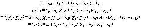
The b0
drops out, but all the other b's (the slopes) retain their identities, so this
is an alternative way of estimating the slopes. The equation can be differenced
as many times as necessary to achieve acceptable Durbin-Watson or Durbin's h
statistics. An intercept term (I call it "a") is left in the
differenced equation, even though it doesn't belong there. This is because if
you estimate the regression without an intercept, that imposes the very
unrealistic restriction that the regression line passes through the origin. It
is better to estimate the unrestricted equation, though a is not the same as b0.
Also the u's are different from the (serial correlated) e's.
Undifferenced
regressions with non-stationary data can benefit from the desirable statistical
property of superconsistency. This
means that the estimated coefficients converge to their true, unbiased values
faster than for OLS estimates with stationary data. Superconsistency is a large sample property,
and the dividing line between large and small samples is ambiguous. A sample less than 30 observations is always
"small," but a sample less than 300 observations may not be
"large."
7.
Violations of regression assumptions:
1.
Heteroskedasticity: Regression theory assumes homoskedasticity of regression
residuals, that is, that the residuals have a constant variance, (otherwise the
standard error of the regression would vary systematically.) If you have this,
invoke White's heteroskedasticity consistent covariance matrix to compute the
results. In MicroTSP use the command [LS(H) Y C X Z W] in TSP use [OLSQ
(ROBUST) Y C,X,Z,W ;]. How do you know if you have it? If you don't get the
same answer without White's matrix as with it, heteroskedasticity is the reason
why. There are a battery of statistical hypothesis tests available to test for
heteroskedasticity, but it's much easier to estimate the regression both
ways. MS Excel 97 does not provide this.
2.
Serial correlation (or Autocorrelation): Use the Cochrane-Orcutt correction in
MicroTSP: [LS Y C X Z W AR(1)]. If necessary, add AR(2) or more terms as well.
When the Durbin-Watson statistic goes close to two, this problem is solved. You
can also difference the equation, see section 6. In TSP use the Beach-MacKinnon
iterative maximum likelihood technique: [AR1 Y C,X,Z,W ;], but usually this
only works for annual data because you can't add more terms if you need to.
With cross-sectional data, just change the order of the data, (you can do this
as long as the order doesn't matter.) MS Excel 97 does not provide this.
3.
Multicollinearity (1): Some of your variables are too similar for the computer
algorithm for minimizing the sum of squared residuals (e'e) to handle.
You'll get an error message regarding a "near singular matrix" which
the computer can't invert (see section 8 below). Excel returns the LINEST
function. There are two possibilities:
a. It is
an exactly singular matrix (the computer can't tell the difference)
because you have accidentally entered the same variable twice in the same
regression. Look for the left-hand-side variable on the right, or one of the
right-hand-side variables repeated. Excel's LINEST function error message
indicates the regression cannot be computed because one variable is a linear
function of another. One of the few advantages of MS Excel 97 is that Excel
is so user-hostile it is very difficult to make this mistake.
b. One
(or more) of your variables is very much smaller in relative magnitude than the
rest. This is called a scale problem. The computer treats it as a string of
zeroes, and it's a linear function of the string of ones it uses for the
constant. You can tell if you have this by plotting all your data together: in
MicroTSP the command is: [PLOT Y X Z W]. In MS Excel 97, plot your data by
clicking on the "chart wizard" icon on the standard toolbar. It
looks like a bar chart. If one variable is just about always equal to
zero on the plot, then you should select some time period and divide each
variable by its own value for that time period. This is called indexing, and
should remove any scale problems.
4.
Multicollinearity (2): Although the software can successfully perform the
estimate, it is difficult to interpret. (This is a less serious problem.)
Typically you may find that the F statistic is very high (indicating a good
estimate and a good model,) but the t statistics are all very low, (indicating
that many or all of the variables should be removed from the model.) It is O.K.
to remove variables from the model as long as the F statistic remains high (or
its probability level remains low.) If you cannot remove any variables
without hurting your F statistic, just note multicollinearity as the reason why
the t statistics are so low.
5.
Non-normality: Contrary to common opinion, it is not a requirement of the
standard regression model that regression residuals be normally distributed.
However, if they are normally distributed, that guarantees that the residuals
are also homoskedastic and not serially correlated. To test for normality,
calculate the Jarque-Bera efficient normality test statistic. In MicroTSP,
right after you run the regression, use: [HIST RESID] and the Jarque-Bera
statistic will be at the bottom of the histogram, next to its probability
level. J-B tests the null hypothesis of normality. You want the probability to
be greater (not less) than .05, or some other significance level,
otherwise the residuals aren't normally distributed. TSP does this
automatically whenever you estimate a least squares regression, but in MicroTSP
you can test any variable for normality with the HIST command, which is very
convenient. SAS does a different test, the Wilson statistic, with the PROC
UNIVARIATE command. The closer the Wilson statistic is to one, the more nearly
normal the variable being tested. The traditional test for normality, the
Kolmolgorov-Smirnoff test, was difficult to compute, and was invented by two
Russian mathematicians. The Jarque-Bera test was invented by economists. If
your residuals are normally distributed, you can claim that your estimate is
close to the maximum likelihood estimate.
MS Excel
97 does not provide a test for normality, but you can compute skewness and
kurtosis of your residuals with the "Descriptive Statistics" option
in the "Data Analysis" menu. The skewness of the normal
distribution is 0 and the kurtosis 3. Check the "Residuals" box in
the regression dialog box to save your residuals when you run a regression.
8.
Regression computations: (Inverting the matrix). In the general multivariate
regression model, y = Xβ + e, a
least squares regression is performed by calculating an estimate of β, called b. Both b and β are (k+1 x 1) column vectors. The least
squares formula is b = (X'X)-1X'y. The matrix
formulae X'X and X'y are not too difficult to calculate, even
with large numbers of explanatory variables. However, inverting the matrix X'X
to get (X'X)-1 is not easy, and before the days of computers
(up until the early sixties), regressions could not generally be calculated
with more than five or six right-hand-side variables. Even supercomputers have
been known to balk at large inversion problems.
9.
Some alternatives to ordinary least squares: (none are provided by MS Excel
97)
1.
Single equation techniques:
a.
minimum absolute deviation (MAD)
b.
minimum sum of absolute errors (MSAE)
c.
instrumental variables (IV) [You can do this in MS Excel 97, but you have to do
all the work yourself.]
d.
two-stage least squares (2SLS) [This can be done in Excel the same as with
instrumental variables.]
e.
weighted least squares
f.
limited information maximum likelihood (LIML)
g.
full information maximum likelihood (FIML or just ML)
h.
recursive least squares
i.
Kalman filtering
j.
non-linear least squares (NLS)
k.
least median of squares (LMS) [This is an outlier-resistant technique designed
to avoid having the estimate unduly influenced by unusually large or small
observations.]
2.
Simultaneous equation techniques
a.
seemingly unrelated regressions (Zellner's method) (SUR)
b.
limited information maximum likelihood (LIML)
c.
full information maximum likelihood (FIML or just ML)
d.
three stage least squares (3SLS)
e.
generalized method of moments (GMM)