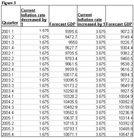
U.S. GDP is forecast to grow 3%  per year from 2001-2005.  The method used to explain the forecast is based on the Phillips Curve.  The Phillips curve indicates the higher the inflation rate the lower the unemployment rate and the lower the inflation rate the higher the unemployment rate.  The forecast assumes that the inflation rate will stay at a constant +1 (1.675) or –1 (3.675) from its current state of 2.675.

This paper forecasts U.S. Gross Domestic Product (GDP) for the years 2001-2005.  The explanatory variable is future inflation forecasted by experts.   The GDP gap is used as the right-side variable.  The gap is the difference between potential GDP and actual GDP.  When actual GDP increases above potential GDP, making the GDP gap negative, unemployment goes down, and producers bid up resource costs to produce the extra output.  When actual GDP decreases below potential GDP, making the GDP gap positive, unemployment goes up, and producers bid down resource costs to produce less output.  The approach is based on the Phillips Curve.  The unemployment variable in the Phillips Curve will signify GDP because of the link between the two.  If unemployment is up, GDP is down and if unemployment is down, GDP is up.

The Gross Domestic Product is the best measure of our national income and output.  Forecast GDP decline could mean an economic recession.   Because the forecast is for five years the possibility of external factors causing the forecast to be wrong is quite probable.  But the forecast horizon is short enough to minimize likely forecast errors.

The rest of this paper is organized as follows:  part 2.  presents the data used to forecast GDP;  part 3. presents the theoretical basis for the approach adopted in forecasting GDP;  part 4.  presents forecasts of GDP for 2001-2005;  part 5.  evaluates the importance of the forecast for the economy;  part 6.  discusses conclusions for economic policy.

The variables used are from the Federal Reserve Bank of St. Louis Federal Reserve Economic Data (FRED).  The measures of real GDP, potential GDP, and forecast inflation are taken from FRED and have the variables GDPC1, GDPPOT, and PHIL.   Both GDPC1 and GDPPOT are measured in chained 1996 dollars.  The inflation data comes from the Federal Reserve Bank of Philadelphia Inflation Survey, also known as the Livingston Survey.  All the variables are given quarterly.  Data were taken starting from the first quarter of 1990, ending with the fourth quarter of 2000 to forecast GDP from 2001 to 2005.

GDP was used because it is the best indicator of our nation’s well being, by simultaneously measuring income, output and expenditures.   Alternative measures were considered such as GNP, real net private income, and real disposable income, and any could have been used in this case, but these are narrower measures of economic performance. The potential and actual GDP data was used in calculating the GDP gap.

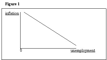
The Phillips Curve indicates that as inflation increases, unemployment decreases.  The relationship between inflation and unemployment is shown on the following Phillips Curve chart:
 

The GDP gap is used as the right-side variable to calculate the GDP forecasts.  The GDP gap is defined as the difference between actual GDP and potential GDP.  The following is the formula for the GDP gap:

The GDP gap is forecasts based on the inflation rate.  Once the GDP gap is forecast, subtracting it from the potential GDP leads to the forecast GDP.

These theories and methods make it possible to assume that if inflation decreases then GDP increases.  GDP gap was assumed to be a linear function of expected inflation.

A forecast of future forecast GDP gap was obtained by substituting alternative hypothesized inflation expectations into this estimated equation.

Regression produced the following data:
 

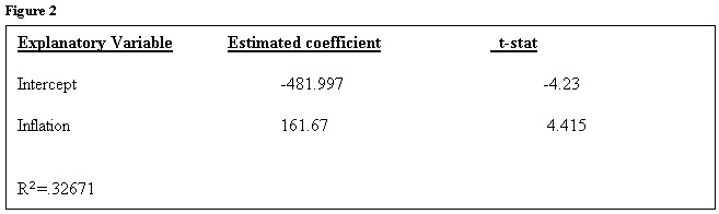
The following table shows the results received:
 

Because it is the best measure of the nation’s level of output, whether good or bad, GDP gives us the best the best measure of the state our economy is in.  This forecast is favorable for the U.S. economy.  Whether inflation goes up or down a moderate amount of  (1%) our GDP is still forecast to increase.  Even though higher inflation tends to cause a bigger percentage rise in GDP, notice the level of GDP is always lower during higher inflation.  If inflation rises by 1% from its current state then the forecast of GDP averages an annual growth rate of  3.05%.  If inflation decreases by 1% from its current state then the forecast of GDP averages an annual growth rate of 2.96%.  This outcome confirms the Phillips curve.

The low inflation in the past couple of years has given us about a 3-4% annual increase in GDP.  This looks like it will continue to rise at about the same rate in the next five years as long as inflation stays within one percent of where it is at this time.

U.S. GDP is expected to rise about 3% annually over the next five years if inflation stays within 1% of its current level.  If the forecast holds true then industries will continue to increase output and workers will continue to have an increased standard of living.  Thus, industries will continue to hire additional workers to continue increasing output.  The Fed should continue to use monetary policy to control inflation.  They should not change interest rates dramatically above or below current levels.  This will allow GDP to grow at its current moderate pace of about 3-4% a year.  This stability in the economy should help the bull market continue, thus causing the wealth effect to continue.  The wealth effect will allow consumers to continue to purchase goods, thus causing manufacturers to continue producing goods.  This will allow a stabile economic cycle.

Federal Reserve Bank of St. Louis, Federal Reserve Economic Data (FRED) http://www.stls.frb.org/fred/, February 1, 2001.

Thomas, Lloyd B., Money, Banking, and Financial Markets, New York: The McGraw-Hill Companies, Inc.,  1997