Topics:
      Review of Problems Sets PS1A & PS1B

      NORMALIZING DATA FOR DESCRIPTIVE COMPARISONS

            What is a Z-value?

      Basis of Inferential Statistics

      Which Statistical Test to Use and When:

           Population Z score
           Sample Z score (variance known in the population)
           Sample t score (variance unknown in the population)

      CONCEPTUALLY:  Evaluating  Computed Stastic / "Standard Error"

      Sampling Distributions
          Comparing Normal to T distribution
      EMPHASIS ON VARIABILITY!

         COMPARING VARIABILITY OF GROUPS

                  BETWEEN / WITHING

      Probability Distributions
        NORMAL DISTRIBUTION
      Statistical Tools: EXCEL FUNCTIONS
           NORMDIST
           Other Normal Distritution functions in EXCEL
      Discussion of Problem Set 2

I.  Basis of Inferential Statistics

            PROBLEMS:

                    What data to monitor
                    How to Obtain Data
                    How to Analyze Data
                    How to Deal with VARIABILITY

 II.  VARIATION

        Variation is a fact of life --- thruth is we have it !,  but what is it?
             In simple terms, Variance is a measure of how scattered the data are due to:
                       Differences
                       Inconsistantcies
                       Changes
                       Volitility
                        etc

                 Types of Variation:

                        Explained Variation
                        Random Variation (unexplained or ERROR)

                 Sources of Variation:

                       People
                       Materials
                       Measurement
                       Methods
                       Machines
                       Environment
                       etc.

 POINT!!!  CONTINUOUS IDENTIFCATION AND REDUCTION OF
                            VARIATION MEANS IMPROVING QUALITY AND PRODUCTIVITY.

III.  DISTRIBUTIONS

       BASIC PROBLEM:  IS THE SAMPLE A "TRUE" REPRESENTATION OF THE POPULATION?

       Must Analyze the stastic based on probablility of chance occurance.

      What is a distribution?

          The grouping  of  data defined by a boundary function curve   f (x).

           For any given group, a unique f(x) or DISTRIBUTION exits,  however
           traditional statatistical theory and approaches have generalized groupings into
           some the following distributions:

                          NORMAL
                            STUDENT'S T
                            F
                            POISSON
                            BIONOMIAL
                            LOGNORMAL
                            CHI SQUARE

              THE ROLE OF PROBABILITY PROVIDES THE BASIS FOR DECISION MAKING.
              THEREFORE, UNDERLYING PROBABILITY DISTRIBUTIONS ARE EMPLOYED.

              WHAT IS AN UNDERLYING PROBABILITY DISTRIBUTION?
 
 

                    P(roll = 2) = 1/36 = .028
                    P(roll = 3) = 2/36 = .056
                    P(roll = 4) = 3/36 = .083
                    P(roll = 5) = 4/36 = .111
                    P(roll = 6) = 5/36 = .138
                    P(roll = 7) = 6/36 = .167

                  THEORETICAL SAMPLING DISTRIBUTIONS:

                   If all parameters are known, no reason to use inferential statistics.  However, if a
                   sample is taken and inference to the population is made, an underlying samplying
                   distrubition is used.

                   CENTRAL LIMIT THEORM:

                         1. Distribution of sample means approaches a normal distribution
                             (even if the population itself is NOT normal).

                         2.  The Mean of Sample Means = m

        3.  The Standard Deviation of  the Distribution of Sample Means is equal to:

        IMPLICATIONS:

               1.  Larger sample sizes reflect more accurately "true" parameters.

               2.  If the population is normallly distributed  then,  theorm hold true
                    for even small samples.

               3.  If the population is NOT normally distributed then large sample
                    sizes are necessary to justify its (Central Limit Theorm) use.
 

NOTE:  DEMO EXCEL EXAMPLE

EXCEL FUNCTIONS

NORMDIST(x, mean, standard_dev, cumulative)
NORMDIST gives the probability that a number falls at or below a given value of a normal distribution.
• x -- The value you want to test.
 
• mean -- The average value of the distribution.
 
• standard_dev -- The standard deviation of the distribution.
 
• cumulative -- If FALSE or zero, returns the probability that x will occur; if TRUE or non-zero, returns the probability that the value will be less than or equal to x.
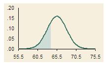
Example: The distribution of heights of American women aged 18 to 24 is approximately normally distributed with a mean of 65.5 inches (166.37 cm) and a standard deviation of 2.5 inches (6.35 cm). What percentage of these women is taller than 5' 8", that is, 68 inches (172.72 cm)?
The percentage of women less than or equal to 68 inches is:
=NORMDIST(68, 65.5, 2.5, TRUE)  =  84.13%
Therefore, the percentage of women taller than 68 inches is 1 - 84.13%, or approximately 15.87%. This value is represented by the shaded area in the chart above.
 
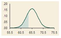
NORMSDIST(z)

NORMSDIST translates the number of standard deviations (z) into cumulative probabilities.
To illustrate:
=NORMSDIST(-1)  = 15.87%
=NORMSDIST(+1) = 84.13%
Therefore, the probability of a value being within one standard deviation of the mean is the difference between these values, or 68.27%. This range is represented by the shaded area of the chart.

NORMINV(probability, mean, standard_dev)
NORMINV is the inverse of the NORMDIST function. It calculates the x variable given a probability.
To illustrate, consider the heights of the American women used in the illustration of the NORMDIST function above. How tall would a woman need to be if she wanted to be among the tallest 75% of American women?

Using NORMINV, she would learn that she needs to be at least 63.81 inches tall, as shown by this formula:
=NORMINV(0.25, 65.5, 2.5)  = 63.81 inches
The figure shows the area represented by the 25% of the American women who are shorter than this height.
 
NORMSINV(probability)
NORMSINV is the inverse of NORMSDIST function. Given the probability that a variable is within a certain distance of the mean, it finds the z value.
To illustrate, suppose you care about the half of the sample that its closest to the mean. That is, you want the z values that mark the boundary that is 25% less than the mean and 25% more than the mean.
The following two formulas provide those boundaries of -.674 and +.674, as illustrated by the figure.
=NORMSINV(0.25)
=NORMSINV(0.75)

STANDARDIZE(x, mean, standard_dev)
STANDARDIZE returns the z value for a specified value, mean, and standard deviation.
To illustrate, in the NORMINV example above, we found that a woman would need to be at least 63.81 inches tall to avoid the bottom 25% of the population, by height. The STANDARDIZE function tells us that the z value for 63.81 inches is:
=STANDARDIZE(63.81, 65.5, 2.5)  =  -0.6745
We can check this number by using the NORMSDIST function:
=NORMSDIST(-0.6745) = 25%
That is, a z value of -.6745 has a probability of 25%.

NOTE:  WE COULD USE THE EQUATIONS SHOWN BELOW  FOR THE NORMAL DISTRIBUTION AND CALCULATE P(X) FOR DESCRETE X VALUES, USE  DISTRIBUTION TABLES, OR USE THE FUNCTIONS EMBEDDED IN EXCEL!

http://www.statsoft.com/textbook/sttable.html

NOTE:  NEXT WEEK "T-TESTS"