Feedrate = 10 ipm RPM = 2500
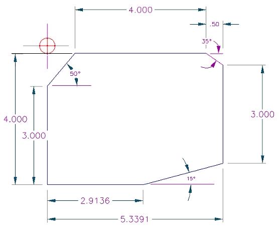
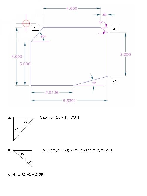
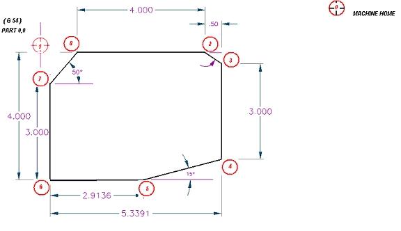
Diagram showing target tool path points.
Introduction
Syllabus
Scope of Course
CNC Basics
Coordinate systems and positioning
methods
NC "Words"
X, Y, Z
F
S
Basic G & M codes
ASSIGNMENTS
Controller Layout
Navigating through MENUS
AutoEdit Software
Lab 2 Prep work
Fixturing and Tooling considerations
Set Up Sheets and Operator Procedures
HAAS VF-1 Introduction
Controller
Layout
Navigating through MENUS
Setting Workplanes G54
Setting Tool Offsets
Manual
calculations for contouring
Trigonometric Functions
Determining Cutter Compensation
Cutter Compensation Methods
Introduction to Lab 3
Complete the following problem for homework.
1. Show all calculations
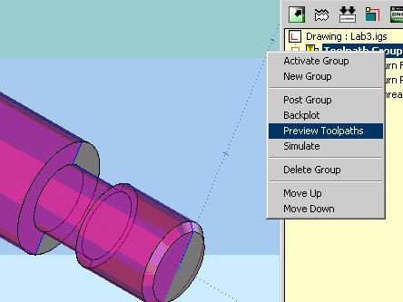
2. Develop required CNC code
3. Simulate tool path in AutoEdit
4. Screen capture simulation graphic
5. Turn in calculations, CNC program listing,
Graphic of tool path
NOTE: Procedures for doing manual calculations
will be explained today, and some of the X,Y coordinates will be determined.
Take good notes!
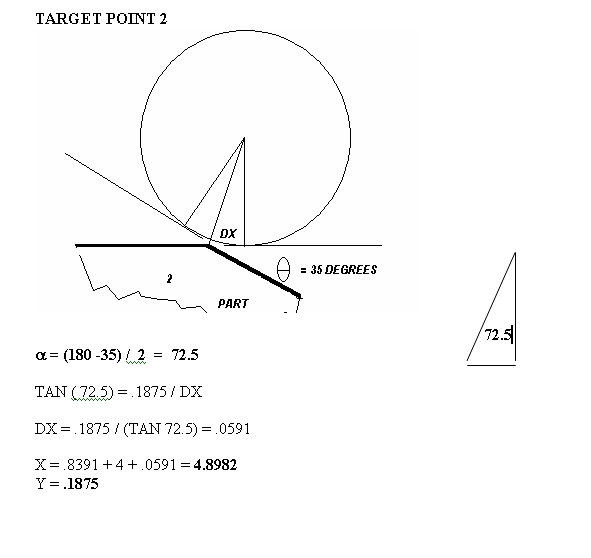
Part to be machined: Cutter: 3/8 Diameter.
Z depth of cut = .1875
Feedrate = 10 ipm RPM = 2500
Diagram showing target tool path points.
FEEDS AND SPEEDS
There are many variables that
affect the speed and feed rates, including:
Type of material
Hardness of material
Condition of material
Type of tool material
Geometry of Tool
Type of Machining Operation
Rigidity of Machine
Rigidity of Setup
Type of Coolant
In general, referenced speeds
and feed data are for beginning points. Adjustments
may be necessary to compensate
for the variables above. Make sure referenced
data matches the type of operation
and variables show above as closely as possible.

NOTE: Referenced Speeds are for HHS and only
recommended starting values:
MATERIAL
SFPM
Aluminum and Alloys 200- 300 FPM
Brass
150- 300 FPM
Bronze
200-250 FPM
Cast
Iron
30 (hard) to 150( soft) FPM
Magnesium
300 - 600 FPM
Steel,
Alloy
30 - 90
Steel, Low Carbon
90-120
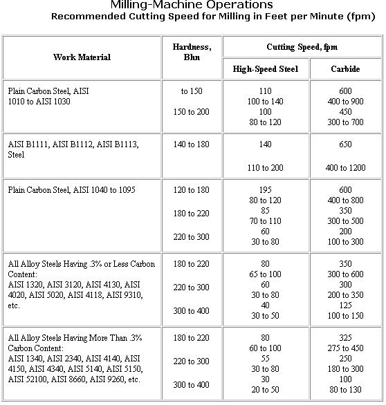
NOTE: A MORE DETAIL CHART CAN BE FOUND AT THE FOLLOWING
WEBSITE: http://www.lexcut.com/catalog/FEEDS-SPEEDS.PDF
A TROUBLESHOOTING GUIDE CAN BE FOUND AT
THE FOLLOWING: http://www.lexcut.com/technical-support.html
Note: General rule
of thumb: Depth of cut should never exceed the radius of the cutter.
SPEED AND FEED RATE CALCULATIONS:
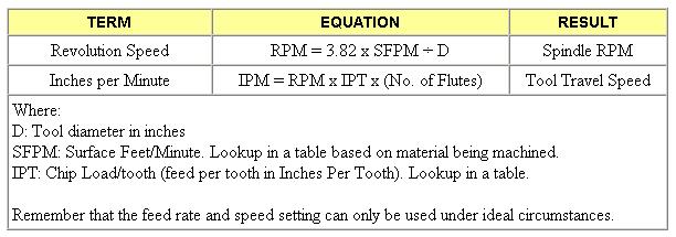
RPM: GENERAL FORMULA:
RPM = CS / CIRCUMFERENCE
ENGLISH: RPM = FT. x 12 in.
x 1 REV
Min.
Ft
p D
METRIC: RPM = m
x 1000 mm x 1 REV
min.
m p
D
NOTE: D = DIAMETER:
FOR TURNING, D = DIAMETER OF STOCK
FOR DRILLING, REAMING, MILLING, D = DIAMETER OF TOOL.
FEED RATES:
TURNING: Refer to Tables for Turning:
MATERIAL
ROUGHING
FINISHING
Cast
Iron
.010 -
.020
.003 - .006
Low Carbon Steel .010 -
.020
.003 - .005
Hi Carbon Steel .008 -
.020
.003 - .005
(annealed)
Alloy
Steel
.005 -
.020
.003 - .005
(normalized)
Aluminum
.015 - .
030
.005 - . 010
Bronze & Brass .010 -
.020
.003 - .010
General Recommendation for low carbon steel: .007 -.010 in. per revolution
(.25 - .4 mm/rev)
is used for roughing. Finishing feeds are .001 - .003 in. per
revolution (.07 - .12 mm/rev)
MILLING: Fr = N x T x RPM
where: N = Number of Teeth
Fr = Feed rate in IPM (or mm per minute for metric)
T = Feed per Tooth per Revolution
RPM = Revolutions per minute = CS/Circumference
MACHINING TIME:
LATHE: MT = LENGTH / (FEED X RPM); MT = L / (F X N)
MILL: MT = LENGTH / (FEED RATE); MT = L / ( fr )
MAKE SURE APPROPRIATE TABLES ARE CONSULTED FOR MATERIAL
AND CUTTING TOOLS BEING USED.
NOTE: THERE ARE TWO TYPES OF MILLING:
UP MILLING (CONVENTIONAL MILLING) - Chips are carried
away from the base stock.
Down Milling (Climb Milling) - Chips are carried into the base stock.
In general,
UP Milling is recommended for older equipment and lower horsepower
machine
tools, and less rigid setups. In climb milling there is a tendency
for the cutter
to
"climb over the work" if the setup is not rigid.
CLASSES OF STEEL
STEEL: PLAIN CARBON
LOW: .10 - .30 % C MEDIUM: .30 - .60 % C HIGH .60 - 1.7% C
ANSI - SAE DESIGNATIONS: 4+ CHARACTERS
(e.g. 1018: first 2 digits classification, last 2 digits %
carbon in hundredths)
x's = % C in hundreths e.g. 10 = .10% Carbon
CARBON STEELS : CLASS [ 1 ]
10xx
Plain Carbon
11xx
Free Cutting Resulfurized
13xx
Manganese
NICKEL STEELS: CLASS [2]
20 xx
.5 % N
21xx
1.5% N
23xx
3.5% N
25xx
5.0% N
CORRISION & HEAT RESISTING: CLASS [3]
303xx
(example)
MOLYBDENUM: CLASS [4]
41xx
Chrominum
43xx
Chrominum Nickel
46xx & 48xx Nickel
CHROMIUM: CLASS [5]
50xx
Low
51xx
Medium
52xx
High
CHROMIUM-VANADIUM: CLASS [6]
6xxxxx
(example)
TUNGSTEN: CLASS [7]
7xxx
(example)
TRIPLE ALLOY: CLASS [8]
8xxx
(example)
SILICON MANGANESE: CLASS [9]
9xxx
(example)
LEADED: NOTE: "L" INDICATES LEADED
11Lxxx
(example)
CLASSIFICATIONS OF ALUMINUM
CODE MAJOR ALLOYING ELEMENT
1xxx
None
2xxx
Copper
3xxx
Manganese
4xxx
Silicon
5xxx
Magnesium
6xxx
Magnesium & Silicon
7xxx
Zinc
8xxx
Other Elements
LETTER DESIGNATIONS:
F As
Fabricated
O
Annealed
Softest Temper
H
Strain
Hardened
H1 Strain Hardened Only
H2 Strain Hardened and
Partial
Anneal
H3 Strain Hardened and
Stabilized
EXTENT OF HARDESS
2 1/4 Hard
4 1/2 Hard
6 3/4 Hard
8 Full Hard
9 Extra Hard
EXAMPLE: 5056-H18
50 Aluminum Magnesium Alloy
56 .56 pure Aluminun
H1 Strain Hardened
8 Full Hard Temper
WEEK 5
Introduction
to ONECNC
Procedures
for importing files
Steps in
creating CNC operations
2D vs. 3D
machining
3D Models
to 2D Engineering Drawings
Importing
files to OneCNC
Manipulating
Files for CNC
Postprocessing
Files
Transferring
Files to CNC Machines
Verifying
Machined Geometry
Contouring
Pocketing
Drilling
Verifying tool paths
Post
processing procedures
Fixturing and Tooling considerations
Set Up Sheets and Operator Procedures
HAAS VF-1 Introduction
Controller
Layout
Navigating through MENUS
Setting Workplanes G54
Setting Tool Offsets
File Importing
Graphical Simulation
IN CLASS DEMO OF ONECNC
ONECNC: PROCEDURES AND TUTORIAL (LAB 4)
ONECNC: PROCEDURES FOR IMPORTING GEOMETRY
FROM EXTERNAL SOURCES AND TOOLPATH GENERATION FOR A VALV
BODY PART (LAB 5)
MID-TERM EXAM REVIEW
STUDY GUIDE:
1. Be familiar with commonly used G codes; be able to define and recognize.
2. Be familiar with commonly used M codes: be abel to define and recognize.
3. Know coordinate and positioning systems used in CNC milling operations.
4. Be able to calculate:
Feed Rates
RPM
Cutting Speeds
Material removal rates
5.
Be able to determine the toolpath required for producing a piecepart by
calculating cutter compensation (manually). Note review your trig!
6. Be familiar with the general procedures and specifically the following operations in OneCNC:
Pocketing;
Contouring;
Drilling
10. Be able to complete required information (in example dialog boxes) for the above operations.
11. Be familiar with the procedures for importing DXF files into OneCNC
12.
Know the various classifications of metals and be prepared to intrepret
the meaning (e.g. 1018 Steel
or 6061-T6 aluminum.
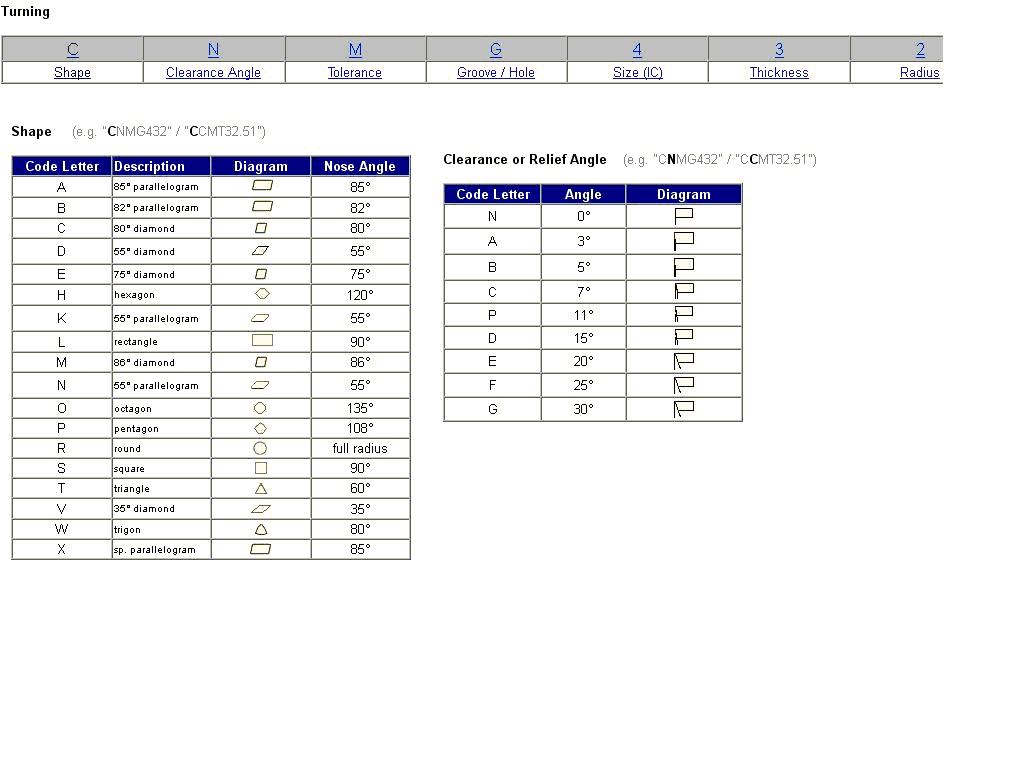
13. Be familiar with ANSI standards for cutting tool inserts.
14. Be familiar the the geometric shapes of commonly used inserts.
15. Be able to sketch a piece part given the CNC code.
16. Know the difference between climb and conventional milling
17. Be able to describe which is preferrable when machining with carbide inserts and why.
18. Be famililar with workplane and tool offsets (HAAS machine)
19. Be familiar with general layout of the HAAS controller (revisit the HAAS website for review)
20. Be able to create a set-up sheet for a piece part
Week 10: MID TERM TEST RETURN AND Work on Aluminum Wallet Designs
Week 11: Production Systems
AUTOMATED MANUFACTURING SYSTEMS
TOPICS:
1. AUTOMATED
SYSTEMS
2. PRODUCTION
OPERATIONS
3. EXAMPLE
PROBLEM
4. HOMEWORK
ASSIGNMENT
5. Project
Discussion & Plan time
DEFINITION OF AUTOMATION: APPLICATION OF MECHANICAL, ELECTRONIC AND COMPUTER BASED SYSTEMS TO OPERATE AND CONTROL PRODUCTION.
FOR THIS COURSE, AUTOMATION WILL BE CONSIDERED AS PERTAINING TO:
PROCESSING
ASSEMBLY
MATERIAL HANDLING
INSPECTION
CIM DEALS WITH THE INFORMATION & SUPPORT OF PRODUCTION
CAD
CAM
CAE
CONTROL
HOW CAN AUTOMATION BE A SUCCESS?
PRODUCT IS STABLE
DESIGNED FOR A SPECIFIC PRODUCT (OR FAMILY)
IS PLANNED AND FLOW IS ANALYZED
SYSTEM IS CAPABLE
SYSTEM IS RELIABLE
ADAPTABLE TO CHANGES IN CUSTOMER NEEDS
TYPES OF PRODUCTION SYSTEMS:
JOB SHOP - LOW VOLUME HIGHLY FLEXIBLE
BATCH - MEDIUM VOLUME ADAPTABLE
MASS - HIGH VOLUME NOT FLEXIBLE
LAYOUTS:
FIXED POSITION - LARGE PRODUCTS (MUST MOVE OPERATIONS TO PRODUCT)
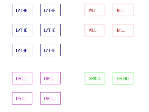
PROCESS - MACHINES ARRANGED AND GROUPED BY TYPE OF PROCESSING
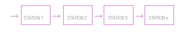
PRODUCT
- MACHINES ARRANGED TO ACCOMMODATE A SPCIFIC PRODUCT OR FAMILY
(FLOW PROCESSING).
Manufacturing Production Systems
TERMS:
Transfer Line
Flexible Manufacturing Systems
Job Shop
Process Layout
Product Layout
Cellular Layout
INTRODUCTION
As a greater demand for a larger variety of products grows, and the increase in global competition for world markets increases, the efficiency in design, production, and delivery becomes critical for the survival of manufacturing firms. Flexibility has become the key ingredient for success and has been possible largely due to advances in computer technology. In this module we will begin with a broad overview of the functions of CAD, CAM, and Manufacturing followed by the comparison of production systems, and finally, an introduction to programmable automation. This topic will be the focus for the remaining class meetings and will deal primarily with control at the machine and workstation level.
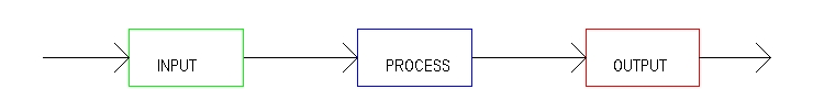
Production Systems Overview: In its basic form, a production
process is simply a system that converts raw materials into useful
products. Usually the system approach is either changing the properties
of a raw material or combining different components to make a final product
that is acceptable to the customer. However the manufacturing cycle,
coordination of data, and system control can become complex across different
types of production systems.
Two main factors must be established before a firm can gain significant
ground in picking up a share of the market and remaining competitive.
Efficiency and Flexibility. In other words, the raw materials
must be available in time (theoretically no sooner or no later than needed)
and flexibility to rapidly change production from one product to another
must be in place. The greatest influence in how these factors come
about in the integration of computers for design (CAD) manufacturing,
(CAM) and control (e.g. CNC and PLC). CAD to CAM to Manufacturing.
The basic functions are shown below:
CAD
Engineering Documentation
Process Requirements
Material Requirements & FEA
Testing and Simulation
CAM
PRODUCTION SYSTEMSProduction Engineering
Tool Design
NC/Control
Process Planning
GT PlanningManufacturing Engineering
Scheduling and Control
Production PlanningQuality Engineering
Process Capability
ReliabilityMANUFACTURINGFabrication
Assembly
Quality Assurance
Production and System Control
Production systems are classified by the arrangement of departments and processing within manufacturing facilities. While many variations can exist, typically there are three major classifications including: 1) Job Shop, 2)Batch Production, and 3) Mass Production. A brief overview along with advantages and disadvantages will be presented.
Job Shop. This type of system is highly customized and produces many different types of products, with very low volume for a given product. A variety of general purpose equipment is used in this environment. Generally speaking, a high degree of skill is required of operators. Machines are typically grouped by type and is referred to as process layout.
A job shop can produce a wide variety of products however, scheduling becomes very difficult to manage from a flow stand point. To give an example of how things can get complicated in a hurry, consider m number of parts being routed through n number of machines. Suppose there are 4 different parts that must be routed through 8 machines. The possible sequences of routing becomes mn or 4 8 = 65,536 possible sequences. It is quite easy to see how this can be a scheduling nightmare.
Batch Production. When products are manufactured in limited quantities, it is referred to as batch production. This type of system is more suited for intermediate size quantities, but those that are not sufficient to warrant a dedicated production line per product. Typically the production capacity is greater than the demand, and products are produced then stored in inventory. Safety stock levels are generated to meet the current and future demand, then production is switched to the next item to be produced to meet scheduling demand. Production equipment and processing machines in a batch environment are more specialized than the job shop. However; the skill level required is decreased. Varying levels of automation exist, and typically machines are arranged in a manner to conform to the products. This type of layout is called product layout.

Mass Production. The mass production system is strictly for
high volume and virtually no flexibility. A production line or even
an entire plant is dedicated to producing only one product. Hard
automation is employed since no changeover is required. Mass production
is capital intensive and requires specialized tooling, jigs, and fixtures.
A high and constant demand is a must for mass production to pay for the
capital invested. Work is moved between stations, and the production
line is balanced to maximize the rate of production. Labor skills
are reduced to a minimum, making work on an assembly line repetitious.
Thus the workstations are good candidates for automation. Two common
terms associated with mass production are assembly line and flow line.
In assembly line production systems workstations are sequential, and parts
are usually moved using conveyors or high speed material handling equipment.
Flow line production is usually associated with processes that are continuous
such as paper, petro-chemicals or continuous casting steel mills.
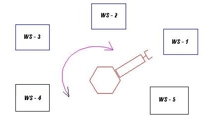
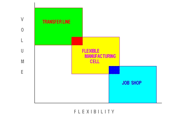
FMS. Across all manufactured goods, batch production is by far the most prevalent. It has been estimated that 95% of all manufactured goods are produced in lot sizes less than an average of 50 parts. Obviously processes layout cannot accommodate high volume, and mass production is not capable of quick changeover. Therefore, cellular or flexible manufacturing systems are require. In this type of system, machines are arranged in a manner to accommodate a "family" of parts within a given group. This is called group technology. By processing similar parts through a cell, set-up times are reduced and throughput times improved. Duplication of equipment and tooling is also reduced.
The diagram shown below illustrates a comparison of job shop, FMS and transfer lines with respect to volume and flexibility.
GOALS:
1.
DEVELOP UNDERSTANDING OF TERMS AND MODELS COMMON TO MFG. SYSTEMS
2. SHOW HOW MODELS CAN BE USED TO EVALUATE SYSTEMS
TERMS STRIVE TO
MLT DECREASE
U INCREASE
PC INCREASE TO COMFORT ZONE (AROUND 95 %)
WIP DECREASE
TIP
DECREASE
MATHEMATICAL MODELS - ASSUME BATCH PROCESSING OF Q PARTS
MANUFACTURING LEAD TIME
MLT IS THE TOTAL TIME TO PROCESS PARTS THROUGH THE PLANT.
nm
MLT
= S
[ Tsui
+ QToi
+ Tnoi]
i = 1
For varying set-up, processing and non-operational times, the average can
be used:
___ __ ___
MLT
= nm [ Tsu + QTo + Tno]
For flow type operations (assuming synchronized):
MLT
= nm (TTR + To Longest)
FOR BATCH PROCESSING:
PRODUCTION TIME:
TP = (TSU + QTO) / Q conceptually TIME / QUANTITY e.g. hrs./piece
PRODUCTION RATE: conceptually QUANTITY / TIME e.g. pices/hr.
RP = QUANTITY / TIME = 1 / TP
PLANT CAPACITY (PC)
PC =[ W (work centers) X SW (shifts/wk x H hours/shifts) x RP (rate of production) ] / nm
UTILIZATION U=OUTPUT / CAPACITY
WORK IN PROCESS (WIP) = [(PC x U / (SW x H)] x MLT
WIP RATIO = WIP / # MACHINES PROCESSING
TIP RATIO = MLT / (nm x To)
= Time to Produce / Actual Operational Time
EXAMPLE INCLASS PROBLEM:
An
average of 20 new orders are started through a certain factory each
month. On average, an order consists of 50 parts to be processed
through 10 machines in the factory. The operation time per
machine for each part = 15 minutes. The nonoperation time per
order at each machine averages 8 hours, and the required setup time per
order is 4 hours. There are 25 machines in the factory, 80% of
which are operational at any time (the other 20% are in repair or
maintenance). The plant operates 160 hours per month.
However, the plant manager complains that a total of 100 overtime
machine-hours must be authorized each month in order to keep up with
the production schedule. Determine the following:
A. What is the manufacturing lead time for a average order?
B. What is the plant capacity (on a monthly basis) and why must overtime be authorized?
C. What is the utilization of the plant?
D. Determine the average level of work-in-process (number of parts-in-process) in the plant.
Solutions:
___
__ __
A. MLT = nm(Tsu + QTo + Tno)
= 10(4 hr + (50 x .25 hr) + 8 hr)
= 245 hours per order.
B. Tp = (Tsu + QTo) / Q = (4 + (50 x .25))/50 = .33 hr./pc
Rp = 1/Tp = 1 / .33 hr/pc = 3.0303 pc/hr.
PC = (Workcenters x Availability x hours/month x Rp) / nm
= (25 x .8 x 160 hrs/month x 3.0303 pc/hr)/10 = 969.7 pc/month
Note: Parts scheduled/month = 20 x25= 1000 pc/month
Schedule exceeds PC by 1000-969.7 = 30.3 parts
Overtime Required = (30.303 pc x 10 machines) / 3.0303 pc/hr =100 hr.
C. U = (1000 pc / 969 pc) = 1.03125 = 103.125%
D. WIP = [(PC x U / HR)] x MLT
= [(969.7 pc/mo. x 1.03125)/ 160 hr/mo] x 245 hr. = 1531.25 pieces
HOMEWORK: Due next Monday.
1.
A certain part is routed through six machines in a batch production
plant. The setup and operation times for each machine are given
belwo. The batch size is 100 and the average non-operational time
per machine is 12 hours. Determine both the MLT and Rp for
operation number 3.
Machine
Setup
(hrs)
Operation time (min.)
1
4
5.0
2
2
3.5
3
8
10.0
4
3
1.9
5
3
4.1
6
4
2.5
2.
Suppose the part in the previous problem is made in very large
quantities on a production line in which an automated work handling
system us used to transfer parts between machines. Transfer time
between stations = 15 seconds. The total time required to set up
the entire line is 150 hours. Assume that the operation times at
the individual machines remain the same as shown in the table
above. Determine: A. The MLT for a part coming off
the line, B) Production rate for operation 3, C) The Theoretical
production rate for the entire production line.
3.
The average part produced in a certain batch manufcturing plant must be
processed through an average six machines. Twenty new batches of
parts are launched each week. Average operation time = 6 minures;
Average Setup time = 5 hours, average batch size = 25 parts, and
average nonoperation time per batch = 10 hours per machine. There
are 18 machines in the plant. The plant operates an average of 70
production hours per week. Scrap rate is negligible.
Determine the following:
A. Manufacturing Leat Time (MLT)
B. Plant Capacity (PC)
C. Plant Utilization (U)
D. Explain the relationship of nonoperational time and the effect on plant utilization.
Week 12:
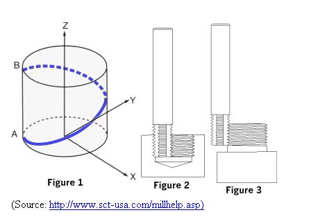
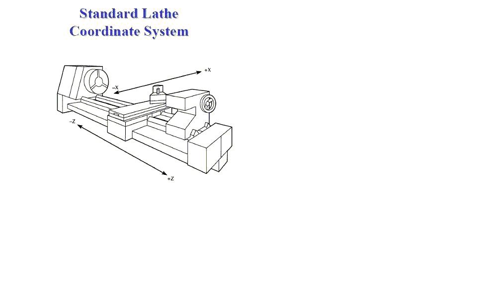
Introduction to CNC Lathe Operations
CNC turning centers,
commonly know as CNC lathes also the Cartesian Coordinate system for
programmed coordinates. However, the axes are different compared
to milling. Only the X and Z axis are used for turning such that
the Z axis represents the center of the spindle and X represents the
tool direction of movement. The diagram below shows the axes for
CNC lathe work.
Objectives: After completing this exercise you should be able to perform the following:
1. Import an IGES file into OneCNC
2. Edit the file for delineating required geometry
3. Set the coordinate system for the lathe operations
(lathe radius)
4. Select the geometry to be turned
5. Specify tooling information required
6. Modify cut control as necessary
7. Generate a tool path for the part specified
8. Post-process tool path for a HAAS lathe
9. Save the file as a PLAIN ASCII format
10. Download file to the HAAS TL-1 lathe
11. Run the program (under supervison) and produce
the required part.
Procedures:
Prior to using OneCNC, create a model or 2D drawing of part shown in the following section. You may create the geometry using a 3D package of your choice (i.e. ProE, ProD) or create using AutoCad or equivalent.
Steps necessary for creating a toolpath are provided with graphical
illustrations .
Major steps include the following:
STEPS: ET 349 Lathe 3D Model Import Method
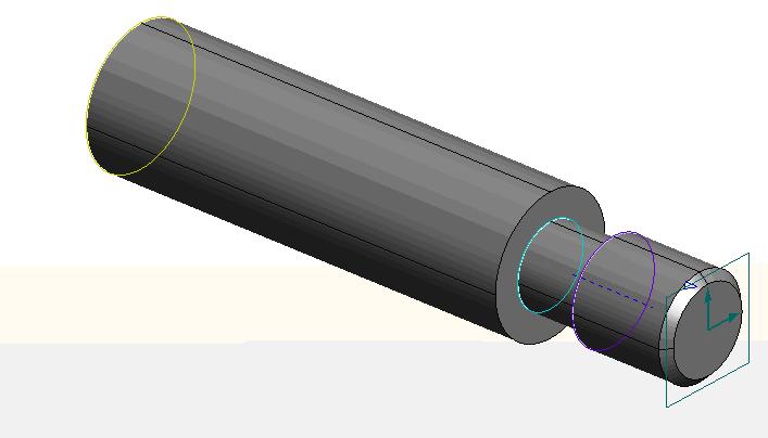
1. Create 3D parametric model. Make sure 0,0,0 is located on the
right end, at center.
2. Export IGES file
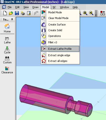
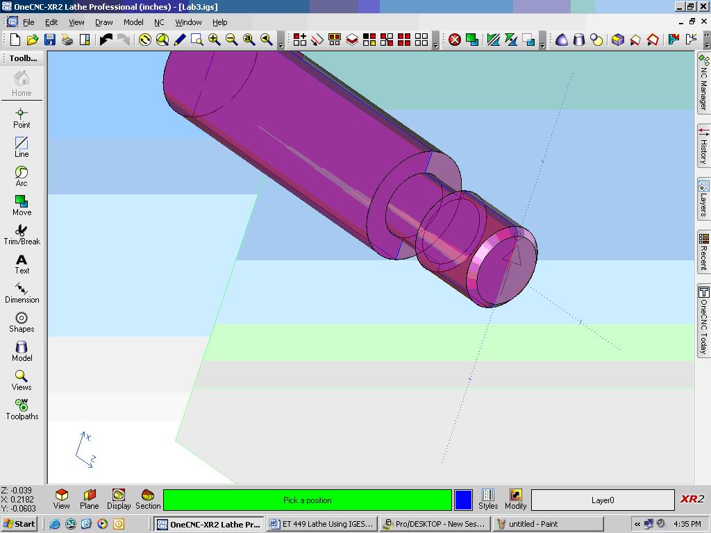
3. Open OneCNC Lathe Professional
4. Import IGES file
5. From the menu, select MODEL: Extract Lathe Profile
6a. A blue outline will be generated representing the lathe profile
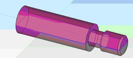
6b. For facing, the line show must be broken and trimmed so facing
will only occur from the center of the part outward (radius).
7. From the Edit menu, select Break, Divide and click on the like as shown in step 6.
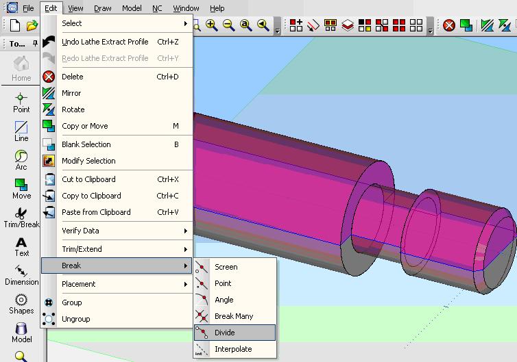
Note: Select the number of divisions = 2.
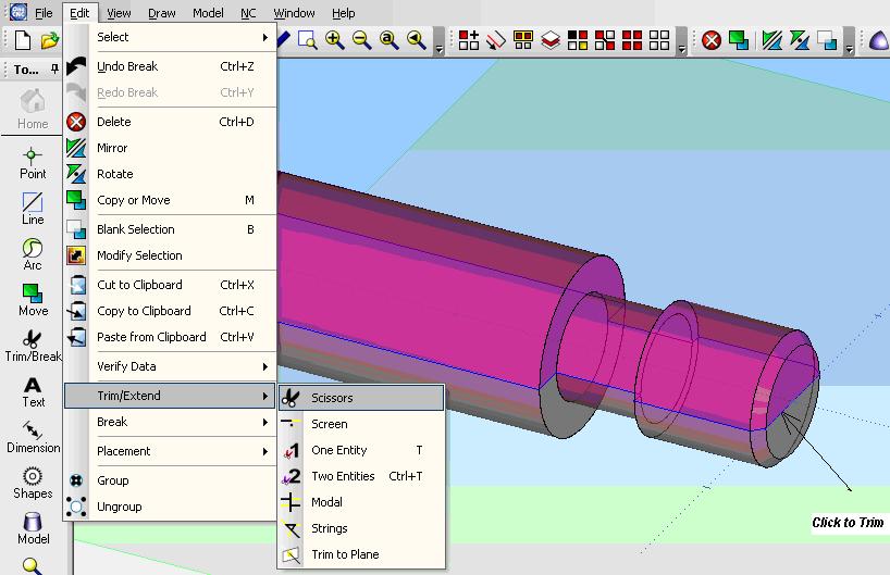
8. Trim the “bottom” half of the line as shown below:
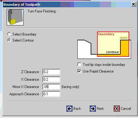
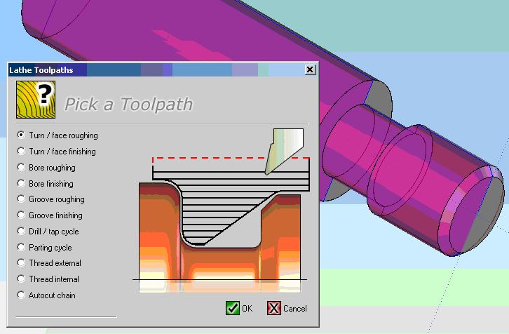
9. Select Lathe Toolpaths and pick Turn/face finishing
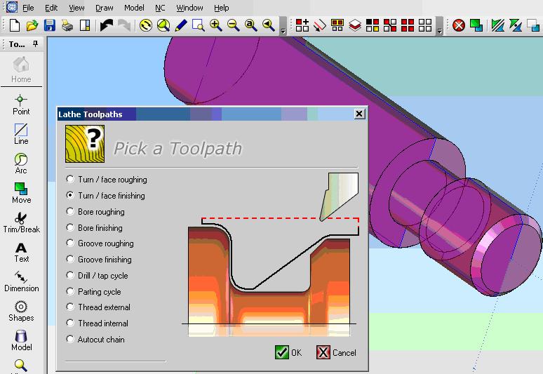
10. Select the line as indicated below for facing, then select end point.
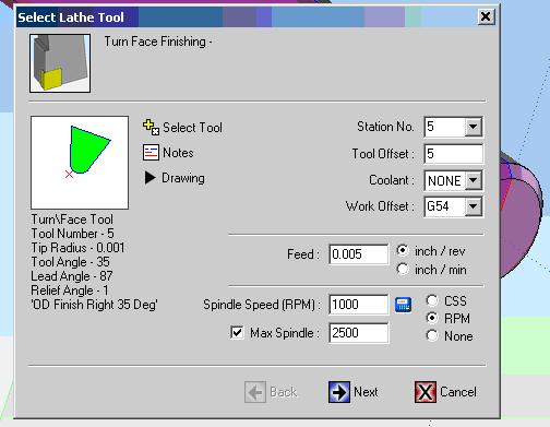
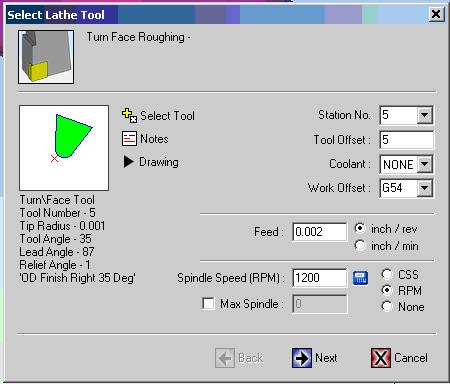
11. Select the tool (for this lab we will use a VNMG 35 degree) tool.
Station should be 5 and tool offset should be 5. Select coolant none
and Work Offset to G54
Specify feed rate for inches/rev between .003 and .005. Select
RPM, Spindle speed = 1000 to 1400 RPM (for acetyl).
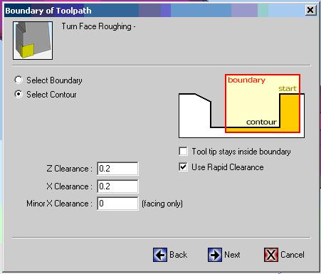
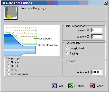
12. Enter values as show for facing operation, then click Next.
13. Enter values as shown in the final dialogue window for the facing
operation.
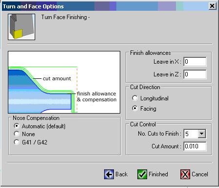
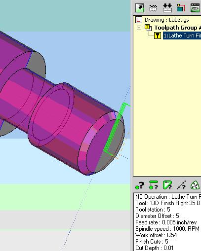
You should now have a toolpath for the facing operation:
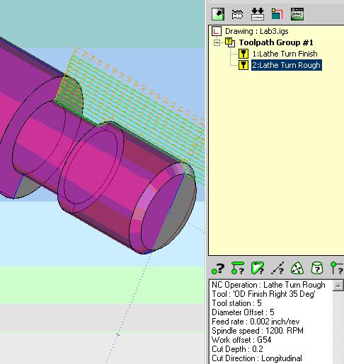
14. Create a ROUGHING operation:
15. Next Pick the profile geometry for the roughing operation as shown
below then right mouse click to select (use the same VNMG tool #5).
16. Enter the values as show on the next two dialogue windows, then
click Finished.
17. You should have a toolpath similar to the one shown below:
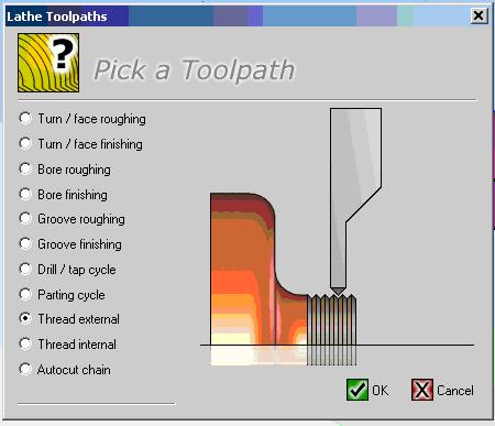
18. Next Create a Threading toolpath: Select External Threading
from the menu as shown:
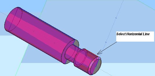
19. Next select the line for the thread geometry as shown:
20. Enter the information in the dialogue windows as shown (note enable
editing
and change the tool information as indicated (change tool angle to
60 deg.)
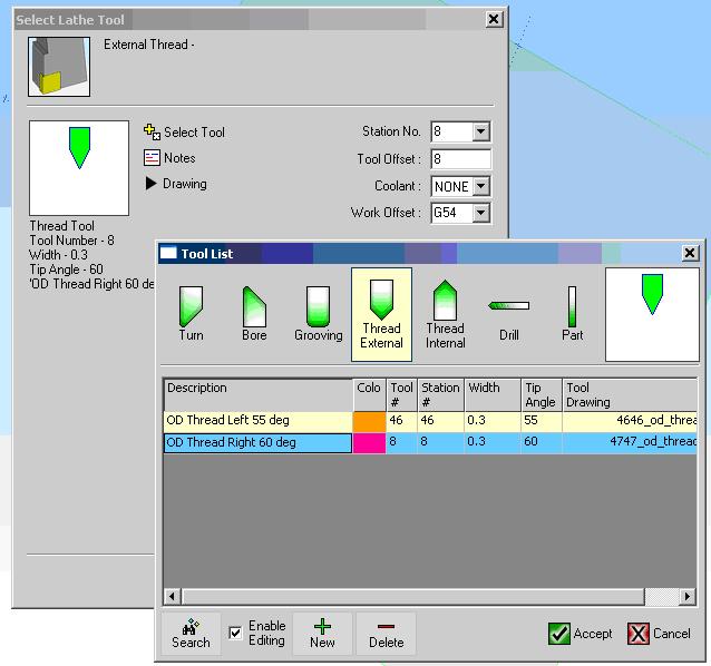
21. Click Accept and verify tooling information is as shown below:
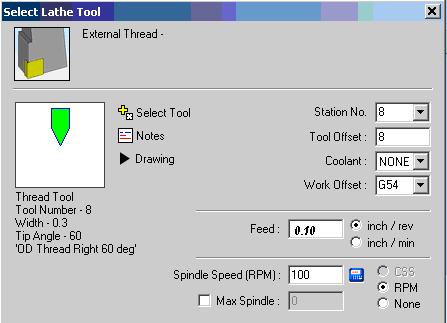
22. On the next screen, enter the information as shown below:
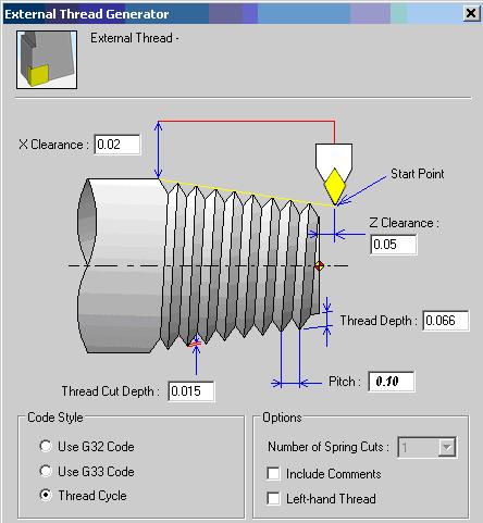
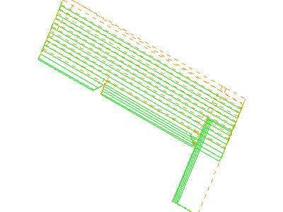
23. Click NEXT, then click FINISHED. You should see a backplot
of the toolpath
similar to the one shown below:
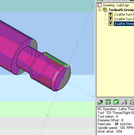
24. Click on NC Manager and select PREVIEW TOOLPATHS. Make sure
TOOLPATH GROUP is highlighted.
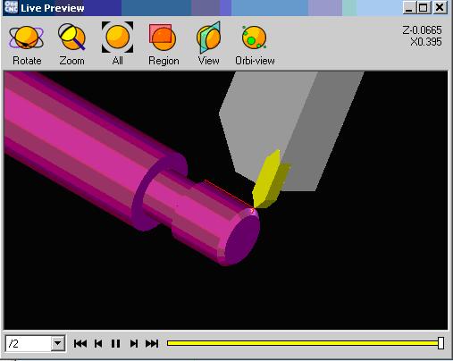
25. You should see a series of tool paths generated on the screen similar
to the ones
shown below:
FACING
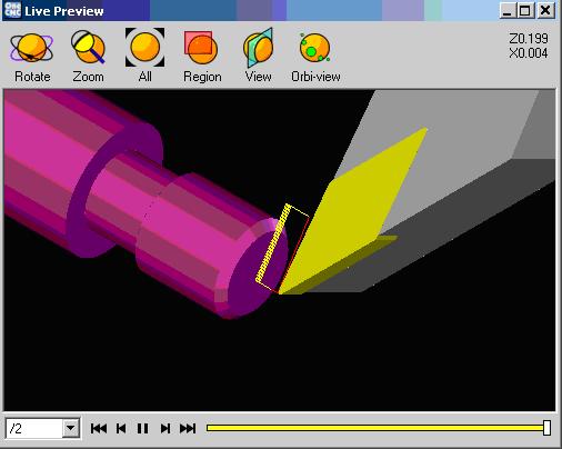
ROUGHING
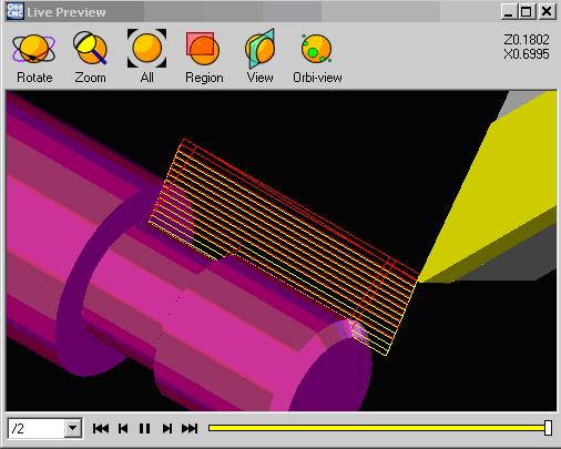
THREADING
26. You are now ready to post process: Make sure HAAS is the post
processor
selected prior to posting as shown: After posting, the file is
ready for download to the HAAS SL20 CNC lathe.
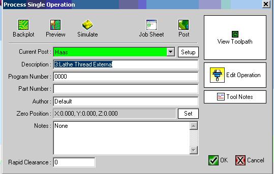
27. You may also want to print a JOB SHEET as depicted below:
JOB SHEET (Toolpath Group #1)
Post Used - Haas
Post Date - Sunday, January 28, 2007 (17:34)
Time to Machine - 25 minutes 52 seconds
Filename - C:\Documents and Settings\ball\Desktop\Lab3.igs
Part Number -
Program Number - 0000
Time of Creation - Sunday, January 28, 2007 16:16
Last Modified - Sunday, January 28, 2007 16:16
System Used - OneCNC-XR2 Lathe Professional - Version 7.33
Author - Default
Notes - None
OPERATIONS
Total number of operations - 3
Operation #1 (1:Lathe Turn Finish)
Operation time - 1 minutes 8 seconds
Tool - Station #5 : OD Finish Right 35 Deg (Turn/Face, 0.38 Dia, 0.00
Tip, F0.005, S1000 RPM)
Operation #2 (2:Lathe Turn Rough)
Operation time - 15 minutes 53 seconds
Tool - Station #5 : OD Finish Right 35 Deg (Turn/Face, 0.38 Dia, 0.00
Tip, F0.002, S1200 RPM)
Operation #3 (3:Lathe Thread External)
Operation time - 8 minutes 51 seconds
Tool - Station #8 : OD Thread Right 60 deg (Thread, 0.30 Dia, 0.00
Tip, F0.1, S100 RPM)
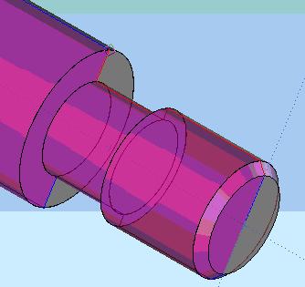
The following part will be produced on a HAAS CNC lathe.
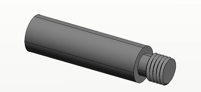
See your lab instructor for assistance in setting up the TL 1.
Machine the part.
Write a report using the standard format.
Threads can be produced in several different manners using CNC machine
tools. Some of these methods include:
A good introduction to threads and fastners can also be found at the following websites:http://www.mech.uwa.edu.au/DANotes/threads/intro/intro.html
http://www.jjjtrain.com/vms/cutting_tools_hand_tap.html#1
Threads can be produced in several different manners
using CNC machine tools. Some of these methods include:
THREAD MILLING: NOTE THAT CUTTER MOVES IN A HELICAL PATH. Any CNC having helical interpolation can cut threads
The next laboratory exercise will cover the steps in producing an
external thread on a CNC lathe.
Purpose: This exercise will cover the basic procedures for Outside Diameter (O.D.) turning and external threading operations in SurfCam. File importing, coordinate systems, CNC options, tool selection, and toolpath generation will be covered.ET 349
CNC LATHE OPERATIONS: O.D. TURNING and External Threading
LABORATORY 7
Objectives: After completing this exercise you should be able to perform the following:
1. Import a dxf file into SurfCam
2. Edit the file for delineating required geometry
3. Set the coordinate system for the lathe operations
(lathe radius)
4. Select the geometry to be turned
5. Specify tooling information required
6. Modify cut control as necessary
7. Generate a tool path for the part specified
8. Post-process tool path for a HAAS lathe
9. Save the file as a PLAIN ASCII format
10. Download file to the HAAS TL-1 lathe
11. Run the program (under supervison) and produce
the required part.
Procedures:
Prior to using SurfCam, create a model or 2D drawing of part shown in the following section. You may create the geometry using a 3D package of your choice (i.e. ProE, ProD) or create using AutoCad or equivalent.
Steps necessary for creating a toolpath are provided with graphical
illustrations .
Major steps include the following:
STEPS:
1. Create DXF
2. Edit and
remove non-essential lines
3. Delete all geometry below the Center Line (C.L.) of the part.
4. Change coordinate system to LATHE RADIUS
5. Move object so that 0,0 is located at the right, C.L. of the part
6. Select NC Lathe
7. Select Turning Option
8. Select geometry to be machined
9. Click DONE and edit tool information
10. Edit Cut Control and turn on undercut
11. Select RETRACT AND CLEARANCE
12. Select OD geometry for threads to be cut
13. Select Threading Tool
14. Edit cut control and select R.H. threading
15. Specify RETRACT AND CLEARANCE
16. Save and transfer to HAAS
17. Produce Part (will assistance from lab instructor)
18. Write lab report and submit
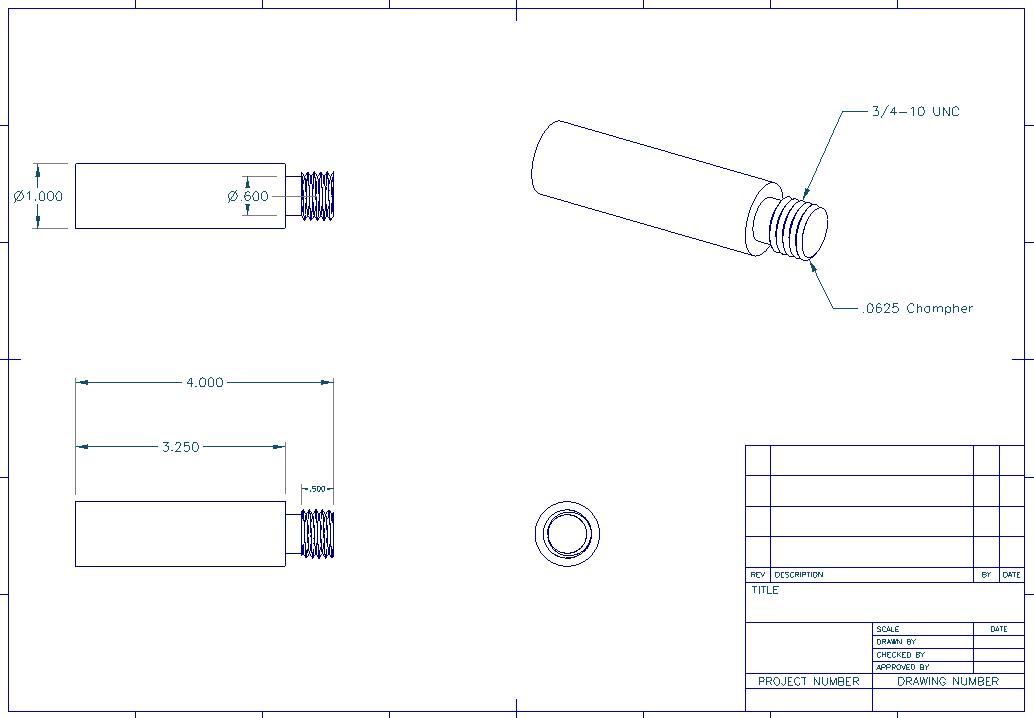
The following part will be produced on a HAAS CNC lathe.
NOTE: Thread Specification: 3/4 -10, UNC, Class 2
Major Diameter: .748
Minor Diameter: .625
Thread Depth: .0615 Depth = (Major
- Minor) / 2
Feed Rate: General Approximation: 1/n or F = P In
this
case F = .1 IPR
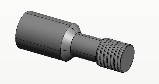
3D - MODEL
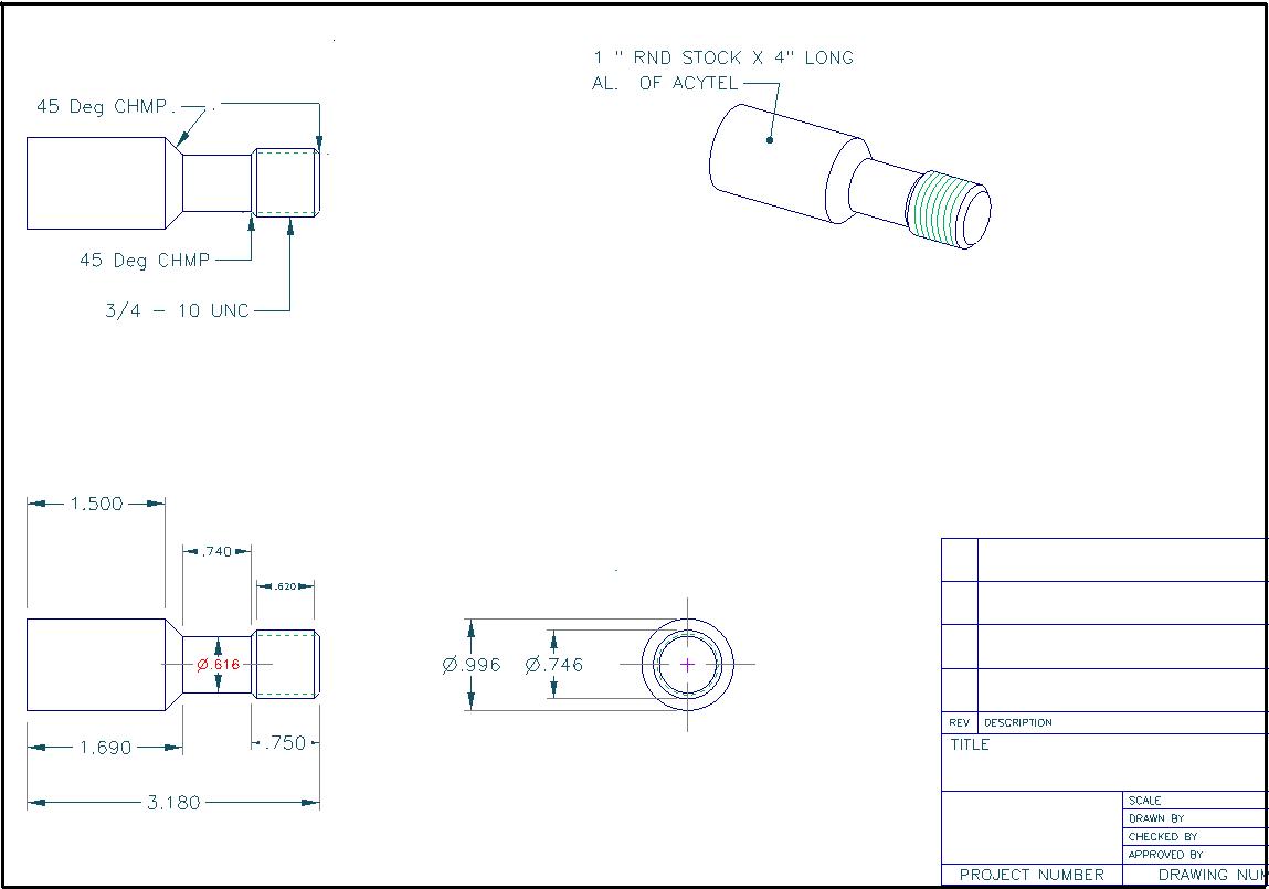
ENGINEERING DRAWING : EXPORT AS DXF